
Sentiment Analysis of IMDb Reviews
Sentiment Analysis Through Natural Language Processing
Sentiment analysis is a method for extracting the sentiment (positive or negative) from natural language. It is an extremely useful tool when it comes to monitoring public opinion, gauging the reception of a firm’s advertisement campaign or, in the case of this project, classifying the sentiment of movie reviews on IMDb. The focus is sentiment analysis of movie reviews, but the principles generalize to all online reviews across most domains. Statistical trends from 2015 show that 90% of consumers read online reviews, and 88% of them trust online reviews as much as personal recommendations. Being able to efficiently and accurately classify the sentiment of online reviews is an invaluable tool for businesses that wish to get ahead of public opinion.
So let’s get to it. For this project I used the data from an old Kaggle competition: “Bag of Words Meets Bags of Popcorn.”, and to spare my machine the time and effort I’ll only be using the training set consisting of 25,000 reviews. This post isn’t meant to be a tutorial so I’m assuming a basic familiarity with NLP and machine learning techniques. Besides the basic formalities of loading in the data our action plan for this project is the following:
- Tokenize the data
- Test/train splits
- Training Word2Vec model using Gensim
- Pre-processing reviews to uniform length
- Create word embeddings using W2V model
- Train a CNN model using the Keras library
The Data
The dataset provided contains three attributes: “id”, “sentiment” and “review”. “Id” shows an anonymized user id within the IMDb website’s database. “Sentiment” is a binary variable classifying the reviews sentiment as positive or negative using the integer 1 or 0 respectively. Finally the actual raw text review is contained in the column “review”. The data contains 25,000 observations of varying review length, with most of them being in the 100-200 word range:

This is going to be a problem later on if we don’t do anything about it. Since we’re training a CNN we will need the reviews to be of equal length so our input arrays all have the same dimension. We’ll cross that bridge when we get there. First thing’s first.
Tokenization
In order for our machines to process the text data contained in the reviews, we’ll need to tokenize it first. We’ll be splitting paragraphs and sentences up into single words, and removing a few commonly used words that don’t tell us much (think of words like “the” and “to”). We’ll do this using gensim’s preprocessing method:
tokens = []
for i in range(0,len(data)):
    temp = []
    temp.append(gensim.utils.simple_preprocess(data["review"][i]))
    temp.append(data["sentiment"][i])
    tokens.append(temp)

# Test/train split

from sklearn.model_selection import train_test_split
train, test = train_test_split(tokens, test_size=0.2)
Clean and simple. While we’re at it we might as well randomly split the data up into training and test samples. The ballpark figure for where to split is said to be around 80/20, so we’ll go ahead with that.
Vector Space
Training the vector space our word embeddings will be living in is also a relatively simple task. So simple that we can do it with a couple of lines:
size = 60
model = gensim.models.Word2Vec ([row[0] for row in tokens], size=size, window=7, min_count=10, workers=10)
model.train([row[0] for row in tqdm(tokens)],total_examples=len([row[0] for row in tokens]),epochs=10)
Gensim’s model is fed the review tokens we made earlier and is trained on those unsupervised. Without going into too many details, it’s going through all of our reviews and clustering words together based on the context they’re used in. The logic being that words used in the same context are similar to eachother. As a simple example think of the words cat and dog. You would assume that they appear in similar contexts since they are both animals and house pets, but not exactly the same since they’re still two distinct species of animal. This would mean that cat and dog would be grouped closer together than say cat and hotdog.
With our W2V model good to go we can move on to some pre-processing.
Uniform Review Length
In this case we want to train a CNN which will require that all our inputs be the same dimension. If you recall review-length distribution from earlier you can see that there is a pretty wide gap between the shortest and longest reviews. In fact the shortest review the shortest review is only 9 tokens long, while the longest is over 2,000. In this case we’ll do some sequence padding. We’ll choose a fixed review length n, and either shorten the review or add tokens containg the word “PAD” to length n:
length = 300
for i in range(0,len(train)):
    if len(train[i][0]) < length:
        for j in range(0,length-len(train[i][0])):
            train[i][0].append("PAD")

    if len(train[i][0]) > length:
        train[i][0] = train[i][0][0:length]

for i in range(0,len(test)):
    if len(test[i][0]) < length:
        for j in range(0,length-len(test[i][0])):
            test[i][0].append("PAD")

    if len(test[i][0]) > length:
        test[i][0] = test[i][0][0:length]
That should take care of our length issues. Let’s take a look at that distribution one more time:

Disclaimer: this is by no means the right way to go about this. We are indiscriminately cutting out words in order for the data to fit out model. Those words contain information that would influence weights of our model, so a more proper approach would be to pre-process the data without having to just omit some of it. It’s possible that simply just vectorizing the data and transforming the data using matrix operations would produce more accurate results, but that’s outside our scope here. Let’s move on to the last steps.
Creating Word Embeddings and training our model
Now our data is almost ready to be fed to the model, but first we need to convert it into something our model will understand. Using our gensim model we’ll convert each word in our reviews into an m dimensional word vector (m=60 in our case):
trainVec = []
testVec = []
for i in range(0,len(train)):
    temp = []
    for j in range(0,len(train[i][0])):
        try:
            temp.append(model.wv[train[i][0][j]])
        except:
            temp.append([0]*size)
    trainVec.append(temp)

for i in range(0,len(test)):
    temp = []
    for j in range(0,len(test[i][0])):
        try:
            temp.append(model.wv[test[i][0][j]])
        except:
            temp.append([0]*size)
    testVec.append(temp)

trainVec = np.array(trainVec)
testVec = np.array(testVec)
After running this we’re good to go. Let’s start building the model:
from keras.models import Sequential
from keras.layers import Dense, Activation, MaxPooling2D
from keras.layers import Convolution2D, Flatten, Dropout
from keras.layers.embeddings import Embedding
from keras.preprocessing import sequence
from keras.callbacks import TensorBoard

net = Sequential()
net.add(Convolution2D(64, 4,input_shape=(length,size,1), data_format='channels_last'))
# Convolutional model (3x conv, flatten, 2x dense)
net.add(Convolution2D(32,3, padding='same'))
net.add(Activation('relu'))
net.add(Convolution2D(16,2, padding='same'))
net.add(Activation('relu'))
net.add(Convolution2D(8,2, padding='same'))
net.add(Activation('relu'))
net.add(MaxPooling2D(pool_size=(3, 3)))

net.add(Flatten())
net.add(Dropout(0.2))
net.add(Dense(64,activation='sigmoid'))
net.add(Dropout(0.2))
net.add(Dense(1,activation='sigmoid'))
net.compile(loss='binary_crossentropy', optimizer='adam', metrics=['accuracy'])

tensorBoardCallback = TensorBoard(log_dir='./logs', write_graph=True)
net.summary()
I won’t go into too much detail about the architecture and kernel dimensions. Suffice it to say this structure gives acceptable results, and is a good starting point towards improving your own state-of-the-art sentiment analysis. I’ll just comment on the one MaxPooling layer for down sampling and the two Dropout layers to prevent overfitting. The model above has just under one million trainable parameters and takes about 20 minutes to train on my machine. With more serious computing power you could easily pump up the number of layers and dimensionality of the data for better results. The chosen model should output a summary like this:

Results
So how does it perform? After three epochs of training we’re able to acheive a training and test accuracy of about 80% and cross-entropy loss of about 43%:
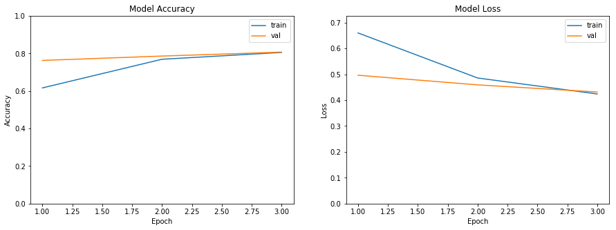
This isn’t that bad considering we’re working with about half of the data available. State-of-the-art performance on a dataset like this is around 89% accuracy. There’s still a ways to go, but like I said this is a good starting point. For further improvement I would suggest increasing the dimensions of the gensim vector space and possibly increase the fixed review length. If you’re interested in the source code then head on over to my GitHub repository.